Understanding unwarranted variations in emergency care

Adventures in Lexicase: Running Time
Population Diversity Leads to Short Running Times of Lexicase Selection
Parallel Problem Solving from Nature
Today I’m sharing a summary of a new paper1 that will be presented at the PPSN conference in a couple of weeks. In it, we prove expected running time bounds on lexicase selection, and in the process, stumble upon a new diversity measure with strong ties to graph theory.
Lexicase selection2 is a parent selection technique that has become very popular in symbolic regression3 and program synthesis4. Part of its appeal is that the algorithm itself is quite simple:
""" lexicase selection of a single individual. """

cases = random_shuffle(cases)

for case in cases:
    if len(individuals) <= 1:
        break

    errors_this_case = [i.error_vector[case] for i in individuals]
    best_val_for_case = min(errors_this_case)

    individuals = [i for i in individuals if i.error_vector[case] <= best_val_for_case]

return random_choice(individuals)
Pseudo-code adapted from PyshGP.
Despite its simplicity, lexicase selection has a few properties that make it very attractive for some problems:
- selection pressure naturally moves to individuals who solve interesting sequences of the training examples.
- selection preserves a high level of useful diversity.
- in many scenarios, individuals can be evaluated lazily on only a small number of examples.
Despite these strengths, one thing that has always been a downside of lexicase is its worst-case complexity. For \(N\) individuals and \(C\) training cases, lexicase selection takes \(O(NC)\) evaluations to select an individual in the worst case. Here, one evaluation means evaluating a single output from a single individual. This complexity dooms a generational evolutionary algorithm (EA) to an overall worst-case complexity of at least \(O(N^2C)\), which is bad (consider tournament selection, which is \(O(NC)\) per generation instead).
In practice, though, the worst case complexity is seldom observed5. Can we say something more formal about the conditions under which lexicase selects individuals more quickly?
In a new paper1, Tom Helmuth, Johannes Lengler and I show that, by measuring population diversity in a graph-theoretic way, the running times of lexicase selection are actually \(O(N+C)\) when diversity is high. And, we see that diversity is quite high in most scenarios where lexicase selection is used.
To prove this result, we needed to think about diversity in a different way.
A Graph-based Diversity Metric
Typically, “diversity” of populations in EAs is measured in fairly simple ways. For example, a measure of behavioral (i.e. semantic) diversity may be the number of unique error vectors in the population; or, for continuous outputs, diversity could be one minus the average pairwise correlation of individuals in the population. However, when understanding lexicase running time, it’s more useful to look at diversity among pairs and clusters of individuals.
Imagine two individuals \(m\) and \(n\) that have made it to some step of a lexicase selection event.
\(\mathcal{C}\) is the set of all cases and there are \(\mathcal{C}'\) cases remaining in the for loop.
For simplicity, assume we have boolean error vectors (error_vector in the code snippet above).
There are interesting things we can say about these individuals.
For example, to have made it this stage of lexicase, they must have identical error on the cases seen so far. What is the probability that, in the next iteration, a case will be drawn on which \(m\) and \(n\) differ, such that one of them is eliminated?
Since cases are randomly drawn each iteration, we can answer this question if we know the fraction of cases on which \(m\) and \(n\) differ. Let’s say they differ on \(\epsilon|\mathcal{C}|\) cases. If we know this, then we know that the probability \(m\) and \(n\) differ on the next case is \(\epsilon|\mathcal{C}|/|\mathcal{C'}|\). Why? \(m\) and \(n\) can only be in the selection pool if all of the cases on which they differ have yet to be visited; those cases are all in \(\mathcal{C'}\).
The key to knowing when lexicase is expected to terminate is knowing the amount by which the selection pool is expected to shrink each iteration (as in drift analysis6). In this example, if \(m\) and \(n\) differ on the next case, we know the selection pool will shrink by at least one. If we could similarly pair up all of the individuals in a selection pool/ the population, we could figure out how the selection pool changes as a whole.
These observations lead us to the following \(\epsilon\)-Cluster Similarity score, for measuring population similarity.
\(\epsilon\)-Cluster Similarity. Let \(\mathcal{N}\) be a population of individuals, and \(\mathcal{C}\) be a set of training cases with discrete losses, for example binary losses. Let \(\epsilon \in [0,1]\). Then the \(\epsilon\)-Cluster Similarity is defined to be the smallest \(k\ge 2\) such that among every set of \(k\) different individuals in \(N\), there are at least two individuals \(m,n\in N\) with phenotypical distance at least \(\epsilon C\).
Let’s unpack this definition a bit. We’ll look at the simple case of boolean errors. Here, phenotypical distance is simply the number of training cases on which two individuals differ. \(\epsilon\) is some fixed fraction so that \(\epsilon C\) defines a number of training cases. So, if we specify a higher \(\epsilon\), we make it “harder” for individuals to be counted as “different”.
\(k\) is the size of a cluster/set of individuals in the population. Importantly, the definition pertains to every possible set of size \(k\). Within each of these sets, there are at least two individuals that differ on at least \(\epsilon C\) training cases. That means that if \(k=2\), every pair of individuals in the population differ on at least \(\epsilon C\) cases. That implies a very diverse population, which is why Cluster Similarity, i.e., \(k\), is low. Conversely, if \(k=N\), we only have one cluster: the whole population. In that case, there only need to be two individuals that differ by \(\epsilon C\). Thus, the population as a whole is very similar: \(N-2\) individuals behave the same on \((1-\epsilon)C\) training cases.
Relation to Graph Theory
If you are familiar with graph theory, you may have come across the concept of the clique of a graph, illustrated below.
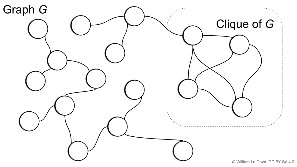
The (maximal) clique of a graph is the largest subgraph for which all vertices are adjacent; i.e., all nodes in the subgraph share an edge. The corresponding clique number is the number of vertices in the clique of the graph.
Let’s define a graph \(G = (V,E)\) where the vertices \(V\) are individuals in our population. We will make an edge between two individuals if they have the same loss on more than \((1-\epsilon)C\) training cases. For such a graph \(G\), \(\epsilon\)-Cluster Similarity is equal to the clique number plus one. Neat!
\(\epsilon\)-Cluster Similarity, which helps explain lexicase selection’s behavior, is a measure of the connectivity of the population when viewed as a graph.
Putting it together
With \(\epsilon\)-Cluster Similarity in mind, we get to our main result.
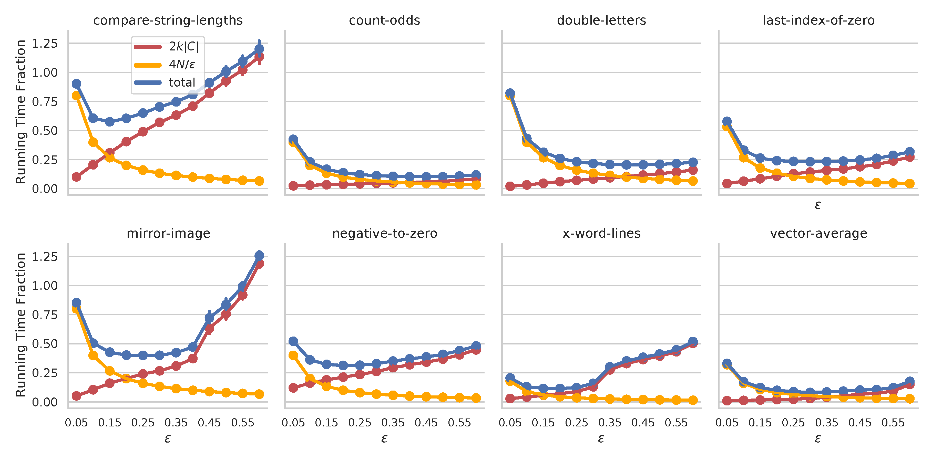
Main Result. Let \(0<\epsilon<1\). Consider lexicase selection on a population of size \(N\) without duplicates and with \(\epsilon\)-Cluster Similarity of \(k\). Let \(M\) be the number of evaluations until the population pool is reduced to size \(1\). Then \[ E[M] \le \frac{4N}{\epsilon} + 2k C. \]
The proof for the main result combines ideas from drift analysis6 with reasoning about the behavior of clusters of individuals during a lexicase selection event. We see there are two additive components to the running-time. The first, \(4N/\epsilon\), relates the fraction of cases, \(\epsilon\), to the population size. Intuitively, if we are lenient about what qualifies two individuals being “different”, \(\epsilon\) is lower and the running time estimate is higher. The second term relates the \(\epsilon\)-Cluster Similarity score, \(k\), to the number of training cases, \(C\). When populations are very similar, \(k\) is high, and the running time is expected to be longer. Both of these scenarios track with our intuition for lexicase selection: with more ties between individuals, fewer are filtered at each stage, and therefore more steps are required in selection.
We illustrate this interplay on 8 program synthesis problems7 below.
Have a gander at our paper to learn more, including results for continuous outputs and for \(\epsilon\)-lexicase selection.
-
Thomas Helmuth, Johannes Lengler, William La Cava (2022). Population Diversity Leads to Short Running Times of Lexicase Selection. Parallel Problem Solving from Nature ↩ ↩2
-
Spector, L. (2012). Assessment of problem modality by differential performance of lexicase selection in genetic programming: A preliminary report. Proceedings of the Fourteenth International Conference on Genetic and Evolutionary Computation Conference Companion, 401–408. http://dl.acm.org/citation.cfm?id=2330846 ↩
-
William La Cava, Lee Spector, Kourosh Danai (2016). Epsilon-Lexicase Selection for Regression. Proceedings of the Genetic and Evolutionary Computation Conference 2016 ↩
-
Helmuth, T., Spector, L., & Matheson, J. (2015). Solving uncompromising problems with lexicase selection. IEEE Transactions on Evolutionary Computation, 19(5), 630–643. https://doi.org/10.1109/TEVC.2014.2362729 ↩
-
William La Cava, Thomas Helmuth, Lee Spector, Jason H. Moore (2019). A probabilistic and multi-objective analysis of lexicase selection and epsilon-lexicase selection. Evolutionary Computation ↩
-
Helmuth, T., & Spector, L. (2015). General Program Synthesis Benchmark Suite. 1039–1046. https://doi.org/10.1145/2739480.2754769 ↩
2025
Taking a closer look at survival modeling with ECGs
2024
Relaxing the definition of equivalent mathematical expressions to get simpler and more interpretable models
2023
About our recent HUMIES award-winning algorithm for clinical prediction models
A new perspective on how this social theory relates to fair machine learning.
2022
We consistently observe lexicase selection running times that are much lower than its worst-case bound of \(O(NC)\). Why?